Response Models

Niek Stevenson

Introduction

This vignette shows how to use the response-only models currently implemented in EMC2. These models fall into two different response geometries:

1. Ordered response models: ordered_probit() and ordered_logit()
2. Multinomial choice models: multinomial_logit() and multinomial_probit()

Ordered response models assume a single latent evidence variable and one or more cutpoints. In the binary case this is the same general setup as signal detection theory: a latent evidence value is compared against a criterion. With more than two ordered responses, the single criterion becomes a set of ordered criteria, as in rating or confidence versions of Signal Detection Theory (SDT). ordered_probit() uses a Gaussian latent noise distribution, which makes it the closest match to classical Gaussian SDT. ordered_logit() uses the same threshold geometry but with logistic noise.

Multinomial response models are different. They are not threshold models on one evidence axis, but random-utility models over a set of alternatives. multinomial_logit() is the standard multinomial-logit or softmax model: each response has a latent utility and the response probabilities are a softmax over those utilities. multinomial_probit() uses the same utility geometry but with Gaussian noise instead of the softmax/logit noise assumption.

The worked examples below use ordered_probit() and multinomial_logit(). The other two models follow the same design logic, but swap the latent noise distribution within the same geometry.

The workflow is the same as for the DDM and race models:

1. Specify the design
2. Inspect sampled parameters and their mapping to design cells
3. Simulate data
4. Define priors and create an emc object
5. Fit the model
6. Summarize posterior estimates and compare observed and posterior predictive choice proportions

choice_summary <- function(data) {
  out <- as.data.frame(prop.table(table(data$S, data$R), 1))
  names(out) <- c("S", "R", "prob")
  out
}

1. Ordered Response Models

Ordered response models place responses on a single latent evidence axis and use cutpoints to divide that axis into response categories. Here we use a 3-category task with low, mid, and high stimuli and responses. location depends on stimulus identity, scale is fixed to 1, and cut ~ 1 estimates the standard K - 1 thresholds.

Conceptually, this is the SDT-like response family in EMC2. In a binary yes/no task there is one criterion. In a 3-category task there are two ordered criteria. location shifts the latent evidence distribution, and cut determines where the response boundaries lie.

matchfun <- function(d) d$S == d$lR

design_ord <- design(
  Rlevels = c("low", "mid", "high"),
  factors = list(subjects = 1, S = c("low", "mid", "high")),
  formula = list(location ~ 0 + S, scale ~ 1, cut ~ 1),
  matchfun = matchfun,
  constants = c(scale = log(1)),
  model = ordered_probit
)

## 
##  Sampled Parameters: 
## [1] "location_Slow"  "location_Smid"  "location_Shigh" "cut_lRlow"     
## [5] "cut_lRmid"     
## 
##  Design Matrices: 
## $location
##     S location_Slow location_Smid location_Shigh
##   low             1             0              0
##   mid             0             1              0
##  high             0             0              1
## 
## $scale
##  scale
##      1
## 
## $cut
##   lR cut_lRlow cut_lRmid
##  low         1         0
##  mid         0         1

sampled_pars() shows the free parameters, and mapped_pars() shows how they map to the latent design cells.

sampled_pars(design_ord)

##  location_Slow  location_Smid location_Shigh      cut_lRlow      cut_lRmid 
##              0              0              0              0              0

p_vector_ord <- sampled_pars(design_ord)
p_vector_ord[] <- c(-1, 0, 1.2, -0.4, log(1.3))

mapped_pars(design_ord, p_vector_ord)

##      S  lR    lM location scale    cut cut_expanded
## 1  low low  TRUE     -1.0     1 -0.400         -0.4
## 2  low mid FALSE     -1.0     1  0.262          0.9
## 4  mid low FALSE      0.0     1 -0.400         -0.4
## 5  mid mid  TRUE      0.0     1  0.262          0.9
## 7 high low FALSE      1.2     1 -0.400         -0.4
## 8 high mid FALSE      1.2     1  0.262          0.9

Now we simulate data from these parameters:

dat_ord <- make_data(parameters = p_vector_ord, design = design_ord, n_trials = 80)

For choice-only models it is often most useful to inspect response proportions directly:

choice_summary(dat_ord)

##      S    R   prob
## 1  low  low 0.7000
## 2  mid  low 0.3500
## 3 high  low 0.0625
## 4  low  mid 0.2625
## 5  mid  mid 0.4750
## 6 high  mid 0.2250
## 7  low high 0.0375
## 8  mid high 0.1750
## 9 high high 0.7125

Next we define a prior and create the emc object.

prior_ord <- prior(
  design = design_ord,
  type = "single",
  pmean = c(
    location_Slow = -0.5,
    location_Smid = 0,
    location_Shigh = 0.5,
    cut_lRlow = -0.2,
    cut_lRmid = log(1.1)
  ),
  psd = c(
    location_Slow = 0.8,
    location_Smid = 0.8,
    location_Shigh = 0.8,
    cut_lRlow = 0.5,
    cut_lRmid = 0.3
  )
)

emc_ord <- make_emc(dat_ord, design_ord, prior_list = prior_ord, type = "single", n_chains = 2)

## Processing data set 1

## Likelihood speedup factor: 26.7 (9 unique trials)

2. Fit the Ordered Model

The following call fits the model and saves the result:

emc_ord <- fit(emc_ord, fileName = "data/response-models-ordered.RData")

summary() reports posterior quantiles, Rhat, and ESS:

summary(emc_ord)

## 
##  alpha 1 
##                  2.5%    50%  97.5%  Rhat  ESS
## location_Slow  -1.596 -0.883 -0.144 0.999 2157
## location_Smid  -0.730 -0.030  0.704 1.000 1871
## location_Shigh  0.566  1.320  2.086 1.000 1974
## cut_lRlow      -1.050 -0.363  0.333 1.000 2155
## cut_lRmid      -0.030  0.167  0.348 1.001 1907

plot_pars() compares the posterior to the generating values:

plot_pars(emc_ord, true_pars = p_vector_ord, use_prior_lim = FALSE)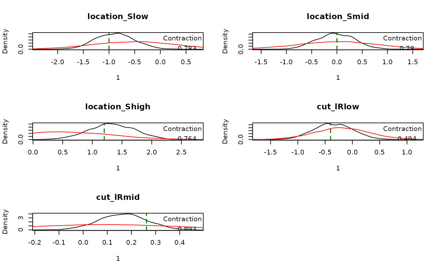

Finally, plot_fit_choice() compares observed response probabilities to posterior predictive intervals:

plot_fit_choice(emc_ord, factors = "S", style = "prob", n_post = 20)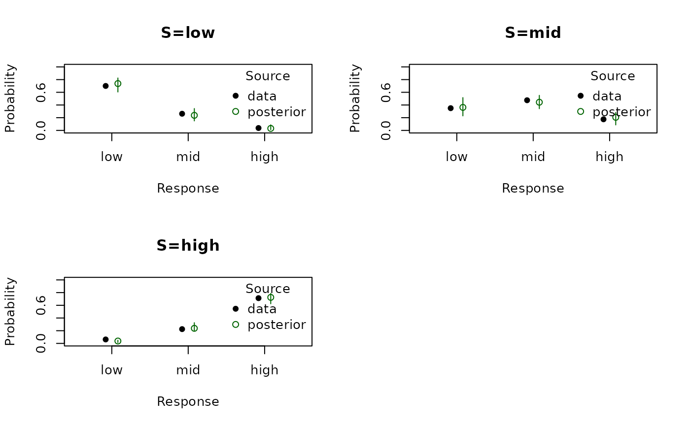

For ordered responses, cumulative fits can also be useful because they reflect the threshold structure directly:

plot_fit_choice(emc_ord, factors = "S", style = "cumulative", n_post = 20)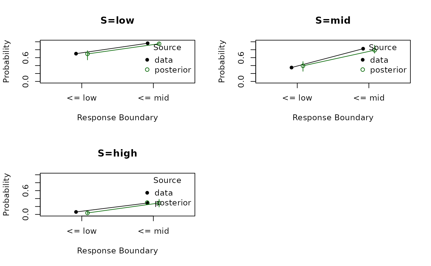

To switch from ordered probit to ordered logit, the design is identical except for the model choice. That is, the latent threshold structure stays the same, but the Gaussian link is replaced by a logistic one:

design_ord_logit <- design(
  Rlevels = c("low", "mid", "high"),
  factors = list(subjects = 1, S = c("low", "mid", "high")),
  formula = list(location ~ 0 + S, scale ~ 1, cut ~ 1),
  matchfun = matchfun,
  constants = c(scale = log(1)),
  model = ordered_logit
)

EMC2 also supports multinomial probit and logit response models, they have documentation, but they mostly exist to be paired with trend models, more on that later!