Race Models

Niek Stevenson

Introduction

This vignette shows a single-subject race-model workflow in EMC2 using the Linear Ballistic Accumulator (LBA). In EMC2, the Racing Diffusion Model (RDM) and Lognormal Race Model (LNR) are also race models and use a similar design logic. Here we use a simulated Stroop task to illustrate how to set this up.

The steps are:

1. Specify a race-model design with multiple responses and stimulus identities
2. Inspect sampled parameters and their mapping to design cells
3. Simulate data
4. Define priors and create an emc object
5. Fit the model
6. Summarize posterior estimates and run posterior predictive checks

For parameter details and transformations, see ?LBA.

1. Specify a Race-Model Design

We define a three-choice Stroop task with stimulus identity S (red, green, blue) and matching response levels. In race models, EMC2 internally builds an accumulator factor lR (one accumulator per response option). We define matchfun to indicate whether the stimulus identity matches each accumulator, which creates the latent match factor lM. By adding S to the drift rate we account for differences in color processing. Similarly, by adding B ~ LR we account for a-priori preferences for responding certain colors.

matchfun <- function(d) d$S == d$lR

# "Average/difference" coding for the TRUE/FALSE lM factor
ADmat <- matrix(c(-1/2, 1/2), ncol = 1, dimnames = list(NULL, "d"))

design_lba <- design(
  factors = list(subjects = 1, S = c("red", "green", "blue")),
  Rlevels = c("red", "green", "blue"),
  matchfun = matchfun,
  formula = list(v ~ lM + S, B ~ lR, A ~ 1, t0 ~ 1, sv ~ 1),
  contrasts = list(v = list(lM = ADmat)),
  constants = c(sv = log(1)),
  model = LBA
)

## 
##  Sampled Parameters: 
## [1] "v"         "v_lMd"     "v_Sgreen"  "v_Sblue"   "B"         "B_lRgreen"
## [7] "B_lRblue"  "A"         "t0"       
## 
##  Design Matrices: 
## $v
##     lM     S v v_lMd v_Sgreen v_Sblue
##   TRUE   red 1   0.5        0       0
##  FALSE   red 1  -0.5        0       0
##  FALSE green 1  -0.5        1       0
##   TRUE green 1   0.5        1       0
##  FALSE  blue 1  -0.5        0       1
##   TRUE  blue 1   0.5        0       1
## 
## $B
##     lR B B_lRgreen B_lRblue
##    red 1         0        0
##  green 1         1        0
##   blue 1         0        1
## 
## $A
##  A
##  1
## 
## $t0
##  t0
##   1
## 
## $sv
##  sv
##   1

design() combines model and experimental structure into an emc.design object.

2. Inspect Parameters and Mapping

sampled_pars() returns the free parameters implied by the design.

sampled_pars(design_lba)

##         v     v_lMd  v_Sgreen   v_Sblue         B B_lRgreen  B_lRblue         A 
##         0         0         0         0         0         0         0         0 
##        t0 
##         0

mapped_pars() shows how those parameters map back to design cells. Here:

• v_lMd captures match-vs-mismatch drift differences
• v_Sgreen and v_Sblue capture stimulus-identity shifts in drift
• B_lRgreen and B_lRblue capture response-specific threshold bias

mapped_pars(design_lba)

## $v 
##   lM     S      
##  TRUE   red    : v + 0.5 * v_lMd
##  FALSE  red    : v - 0.5 * v_lMd
##  FALSE  green  : v - 0.5 * v_lMd + v_Sgreen
##  TRUE   green  : v + 0.5 * v_lMd + v_Sgreen
##  FALSE  blue   : v - 0.5 * v_lMd + v_Sblue
##  TRUE   blue   : v + 0.5 * v_lMd + v_Sblue
## 
## $B 
##   lR     
##  red    : exp(B)
##  green  : exp(B + B_lRgreen)
##  blue   : exp(B + B_lRblue)

In this example we simulate data, but you can replace this with your empirical data. We first define true parameter values on the transformed scale and inspect the numeric mapping:

p_vector <- sampled_pars(design_lba)
p_vector[] <- c(
  v = 1.4,
  v_lMd = 1.8,
  v_Sgreen = 0.15,
  v_Sblue = -0.1,
  B = log(0.7),
  B_lRgreen = 0.1,
  B_lRblue = -0.1,
  A = log(0.3),
  t0 = log(0.25)
)

mapped_pars(design_lba, p_vector)

##       S    lR    lM    v sv     B   A   t0     b
## 1   red   red  TRUE 2.30  1 0.700 0.3 0.25 1.000
## 2   red green FALSE 0.50  1 0.774 0.3 0.25 1.074
## 3   red  blue FALSE 0.50  1 0.633 0.3 0.25 0.933
## 4 green   red FALSE 0.65  1 0.700 0.3 0.25 1.000
## 5 green green  TRUE 2.45  1 0.774 0.3 0.25 1.074
## 6 green  blue FALSE 0.65  1 0.633 0.3 0.25 0.933
## 7  blue   red FALSE 0.40  1 0.700 0.3 0.25 1.000
## 8  blue green FALSE 0.40  1 0.774 0.3 0.25 1.074
## 9  blue  blue  TRUE 2.20  1 0.633 0.3 0.25 0.933

To visualize the implied design-level behavior:

plot_design(design_lba, p_vector = p_vector, factors = list(v = "S", B = "lR"), plot_factor = "lR", layout = c(1,3))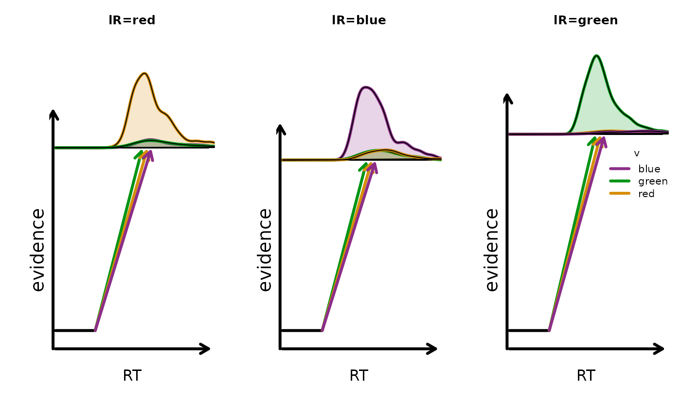

3. Simulate Data

make_data() simulates trial-level responses and response times from the specified design and parameter values.

dat <- make_data(parameters = p_vector, design = design_lba, n_trials = 80)

A quick check of the simulated defective densities by stimulus identity:

plot_density(dat, factors = "S", layout = c(1,3))

4. Set Prior and Build EMC Object

prior() defines prior settings for parameters in this design. As always, be mindful that some parameters are represented on transformed scales, see ?LBA.

prior_lba <- prior(
  design = design_lba,
  type = "single",
  pmean = c(
    v = 1.2,
    v_lMd = 1.5,
    v_Sgreen = 0,
    v_Sblue = 0,
    B = log(0.8),
    B_lRgreen = 0,
    B_lRblue = 0,
    A = log(0.25),
    t0 = log(0.2)
  ),
  psd = c(
    v = .5,
    v_lMd = .6,
    v_Sgreen = .4,
    v_Sblue = .4,
    B = .25,
    B_lRgreen = .25,
    B_lRblue = .25,
    A = .25,
    t0 = .15
  )
)

Inspecting implied priors is a useful sanity check:

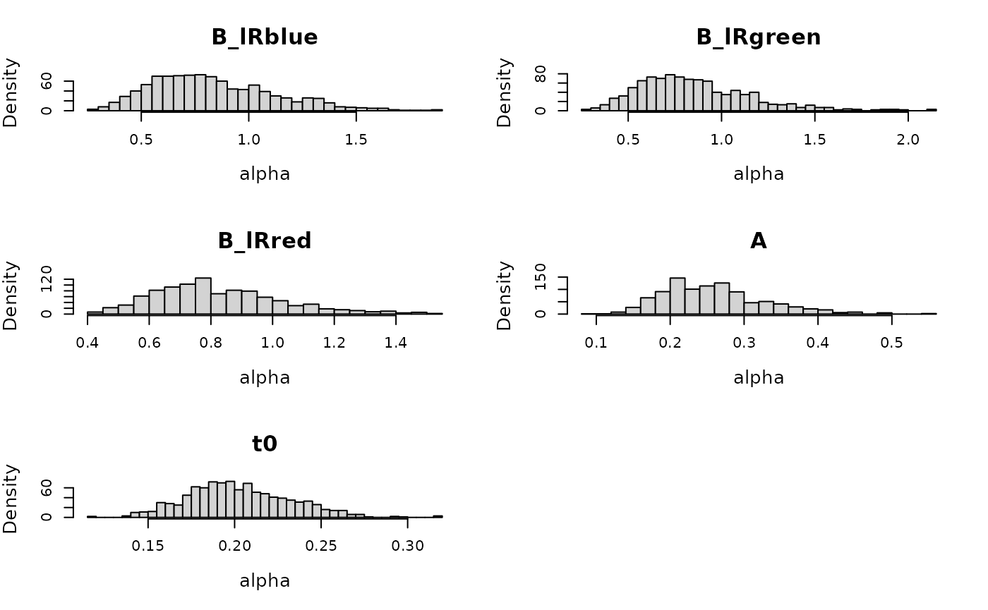
plot(prior_lba, N = 1e3)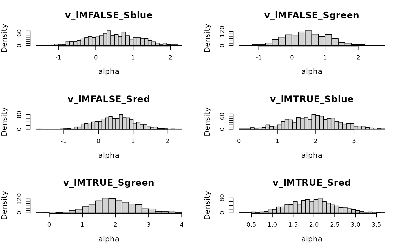

Next we construct the emc object. make_emc() combines data, design, and prior into the object expected by fit().

emc <- make_emc(dat, design_lba, prior_list = prior_lba, type = "single")

## Processing data set 1

## Likelihood speedup factor: 2 (122 unique trials)

5. Fit

The following call is how you can fit this model and save intermediate output:

emc <- fit(emc, fileName = "data/race-models.RData")

6. Summarize and Check Model Fit

summary() reports quantiles, Rhat, and ESS for estimated parameters:

summary(emc)

## 
##  alpha 1 
##             2.5%    50%  97.5%  Rhat  ESS
## v          0.971  1.423  1.850 1.000 2841
## v_lMd      1.622  1.908  2.199 1.000 3000
## v_Sgreen  -0.155  0.159  0.465 1.001 2722
## v_Sblue   -0.432 -0.101  0.197 1.001 2991
## B         -0.592 -0.270  0.007 1.000 2912
## B_lRgreen -0.053  0.071  0.201 1.001 2974
## B_lRblue  -0.206 -0.068  0.060 1.001 2816
## A         -1.897 -1.405 -0.937 1.000 2807
## t0        -1.699 -1.488 -1.320 1.000 3000

plot_pars() compares posterior densities with the generating values:

plot_pars(emc, true_pars = p_vector, use_prior_lim = FALSE)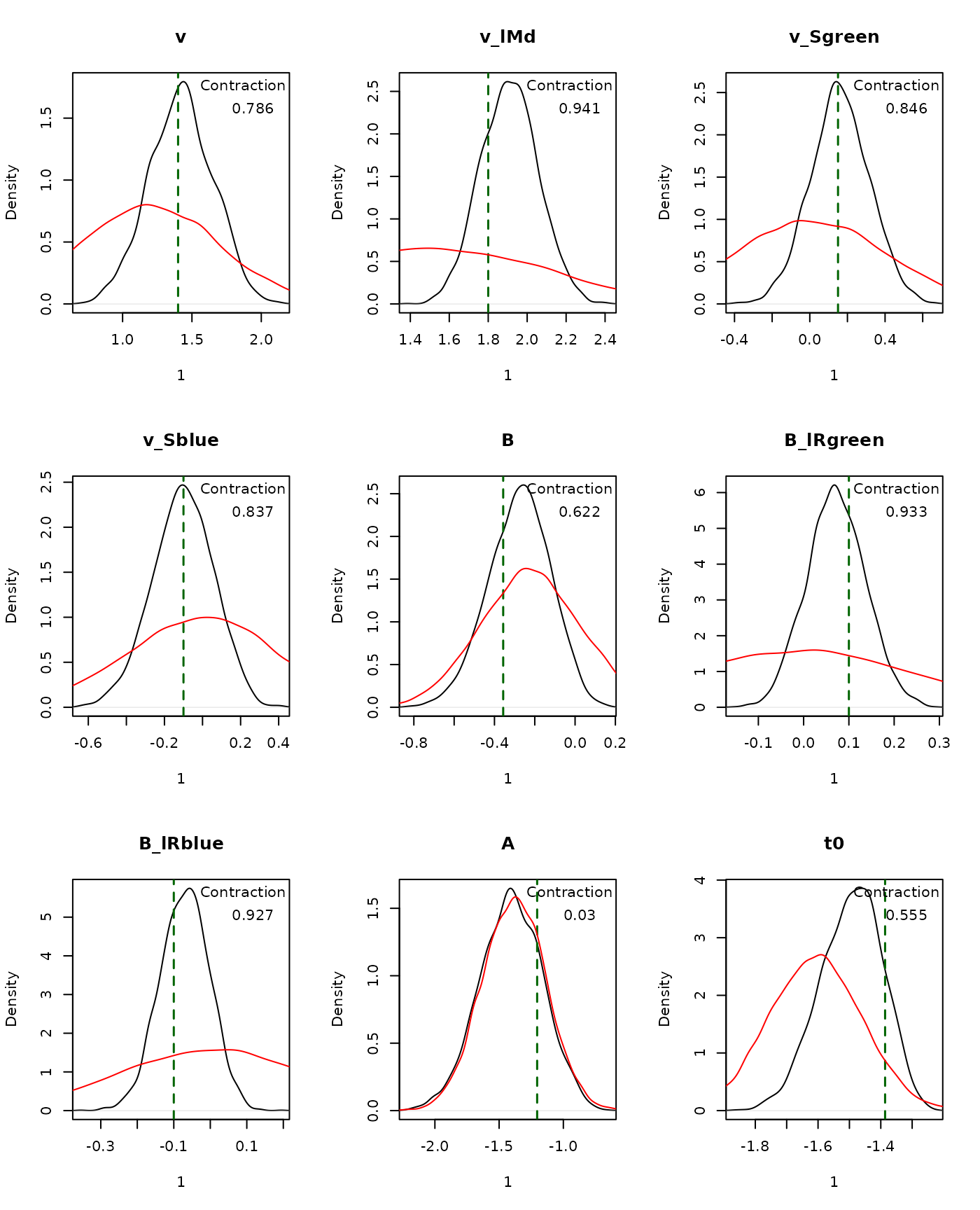

Finally, we generate posterior predictive datasets and compare CDFs:

pp <- predict(emc)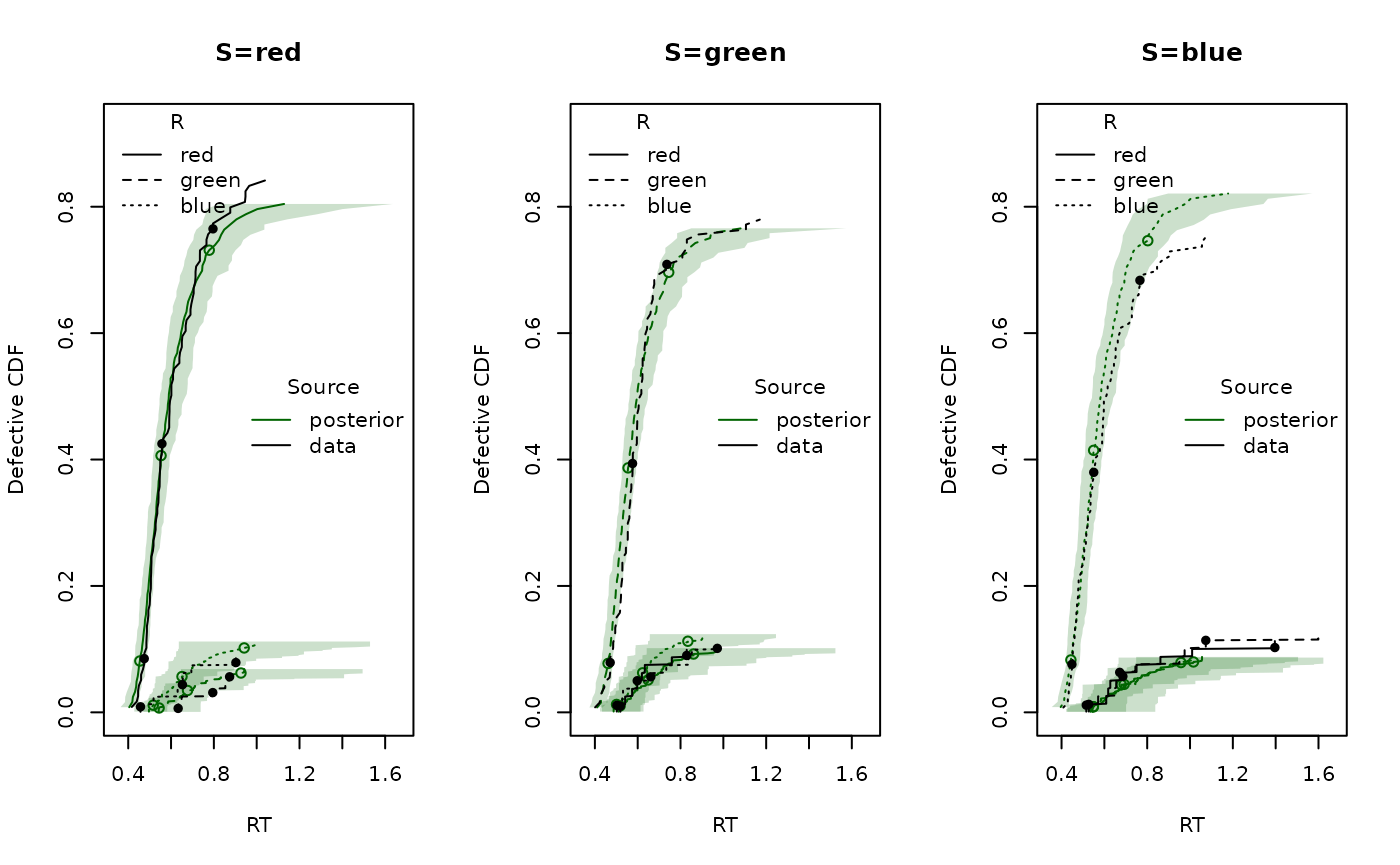

plot_cdf(dat, pp, factors = "S", layout = c(1,3))

This same race-model workflow extends naturally to the other race models RDM and LNR; the core steps (design() -> prior() -> make_emc() -> fit() -> predictive checks) remain the same.