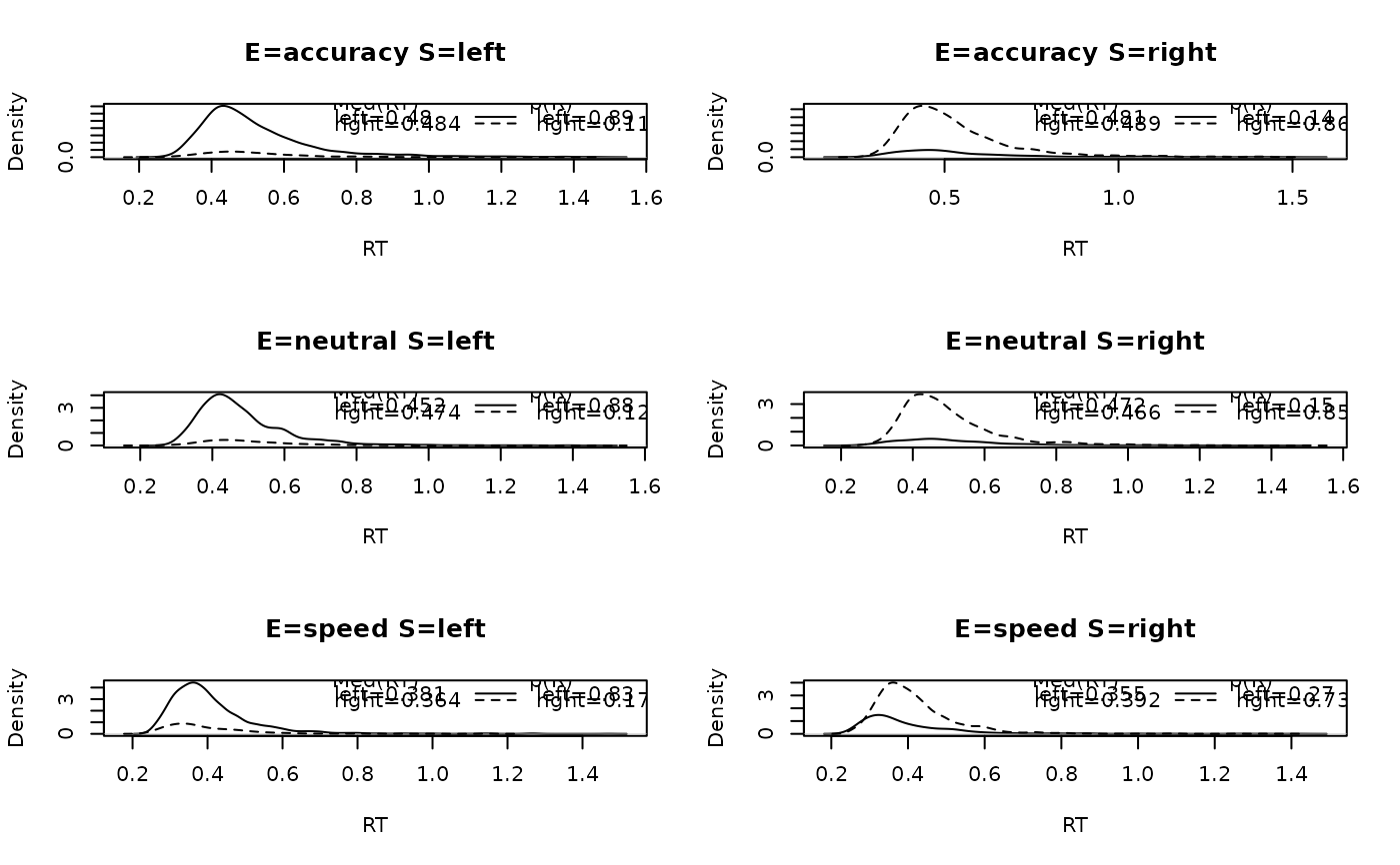
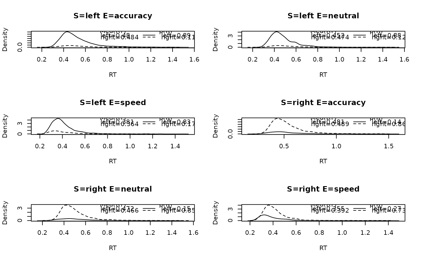
Plot defective densities for each subject and cell — plot_defective

Plots panels that contain a set of densities for each response option in the data. These densities are defective; their areas are relative to the respective response proportion. Across all responses, the area sums to 1.

Usage

plot_defective_density(
  data,
  subject = NULL,
  factors = NULL,
  layout = NA,
  correct_fun = NULL,
  rt_pos = "top",
  accuracy = "topright",
  ...
)

Arguments

data: A data frame. The experimental data in EMC2 format with at least subject (i.e., the subject factor), R (i.e., the response factor) and rt (i.e., response time) variable. Additional factor variables of the design are optional.
subject: An integer or character string selecting a subject from the data. If specified, only that subject is plotted. Per default (i.e., NULL), all subjects are plotted.
factors: A character vector of the factor names in the design to aggregate across Defaults to all (i.e., NULL).
layout: A vector indicating which layout to use as in par(mfrow = layout). If NA, will automatically generate an appropriate layout.
correct_fun: If specified, the accuracy for each subject is calculated, using the supplied function and an accuracy vector for each subject is returned invisibly.
rt_pos: legend function position character string for the mean response time (defaults to top)
accuracy: legend function position character string for accuracy (defaults to topright)
...: Optional arguments that can be passed to get_pars, density, or plot.default (see par())

Value

If correct_fun is specified, a subject accuracy vector is returned invisibly

Examples

# First for each subject and the factor combination in the design:
plot_defective_density(forstmann)

# Now collapsing across subjects:
plot_defective_density(forstmann, factors = c("S", "E"))

# If the data is response coded, it generally makes sense to include the "S" factor
# because EMC2 will plot the "R" factor automatically. This way, choice accuracy can
# be examined
# Each subject's accuracy can be returned using a custom function:
print(plot_defective_density(forstmann, correct_fun = function(d) d$R == d$S))

#>      as1t      bd6t      bl1t      hsft      hsgt      kd6t      kd9t      kh6t 
#> 0.7666667 0.8386337 0.7947805 0.9375000 0.9552415 0.6855124 0.9623086 0.8661888 
#>      kmat      ku4t      na1t      rmbt      rt2t      rt3t      rt5t      scat 
#> 0.8947991 0.7207101 0.9551887 0.8652226 0.9180523 0.7520759 0.6483357 0.7926973 
#>      ta5t      vf1t      zk1t 
#> 0.9195266 0.8436754 0.8114144