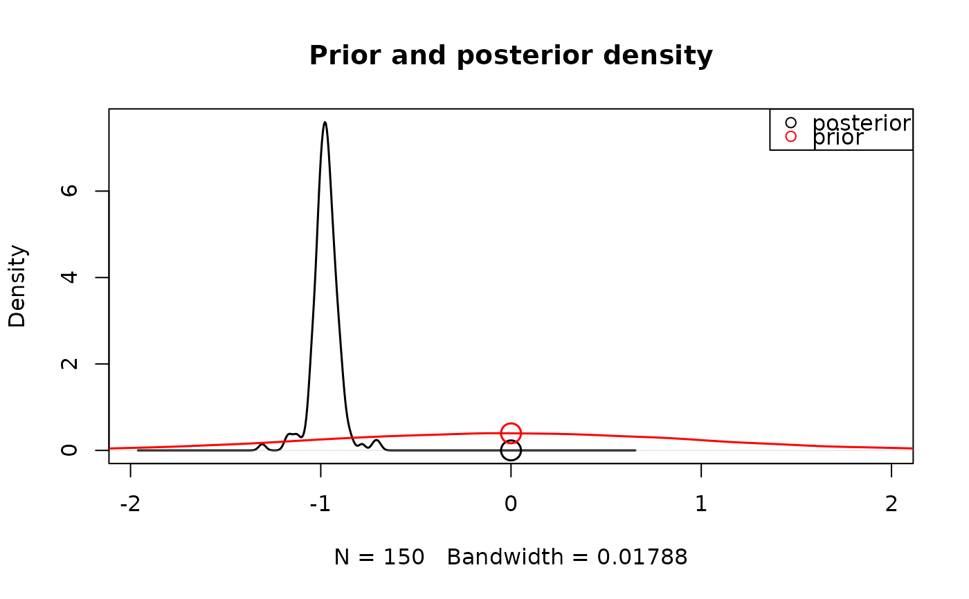
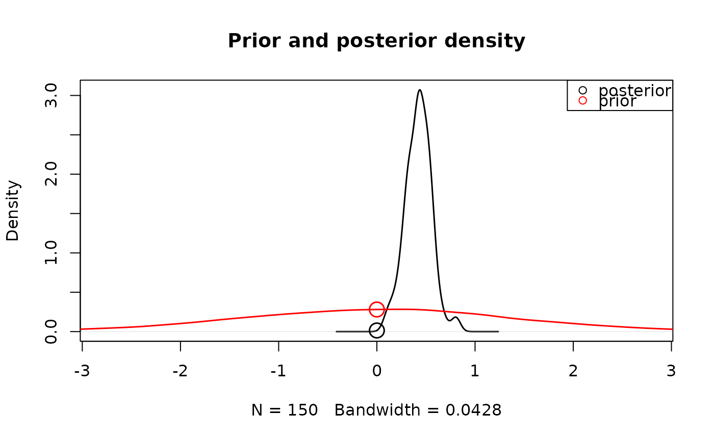
Within-model hypothesis testing — hypothesis.emc • EMC2

Approximates the Bayes factor for parameter effects using the savage-dickey ratio.

Usage

# S3 method for class 'emc'
hypothesis(
  emc,
  parameter = NULL,
  H0 = 0,
  fun = NULL,
  selection = "mu",
  do_plot = TRUE,
  use_prior_lim = TRUE,
  N = 10000,
  prior_plot_args = list(),
  ...
)

hypothesis(emc, ...)

Arguments

emc: An emc object
parameter: A string. A parameter which you want to compare to H0. Will not be used if a FUN is specified.
H0: An integer. The H0 value which you want to compare to
fun: A function. Specifies an operation to be performed on the sampled or mapped parameters.
selection: A Character string. Indicates which parameter type to use (e.g., alpha, mu, sigma2, correlation).
do_plot: Boolean. If FALSE will omit the prior-posterior plot and only return the savage-dickey ratio.
use_prior_lim: Boolean. If TRUE will use xlimits based on prior density, otherwise based on posterior density.
N: Integer. How many prior samples to draw
prior_plot_args: A list. Optional additional arguments to be passed to plot.default for the plotting of the prior density (see par())
...: Optional arguments that can be passed to get_pars, density, or plot.default (see par())

Value

The Bayes factor for the hypothesis against H0.

Details

Note this is different to the computation of the marginal deviance in compare since it only considers the group level effect and not the whole model (i.e. subject-level parameters). For details see: Wagenmakers, Lodewyckx, Kuriyal, & Grasman (2010).

Examples

# Here the emc object has an effect parameter (e.g. m),
# that maps onto a certain hypothesis.
# The hypothesis here is that m is different from zero.
# We can test whether there's a group-level effect on m:
hypothesis(samples_LNR, parameter = "m")

#> [1] 9.952023e+15
# Alternatively we can also test whether two parameters differ from each other
mdiff <- function(p)diff(p[c("m","m_lMd")])
hypothesis(samples_LNR,fun=mdiff)

#> [1] 19.62834